In a recent newsletter John Mauldin wrote: “It is monetary policy madness to raise rates and undertake quantitative tightening at the same time.” However, this is exactly what the Fed plans to do in 2018. Has the Fed gone mad?

If mad is defined as diverging in an irrational way from normal practice then the answer to the above question is no. The Fed is following the same rule book it has always followed.

It should first be understood that earlier rate-hiking campaigns were always accompanied by quantitative tightening (QT). Otherwise, how could the Fed have caused its targeted interest rate (the Fed Funds rate) to rise? The Fed is powerful, but not powerful enough to command the interest rate to perform in a certain way. Instead, it has always manipulated the rate upward by reducing the supply of reserves to the banking system via a process that also reduces the money supply within the economy; that is, via QT. In other words, far from there being something unusual about the Fed simultaneously raising rates and undertaking QT, it is standard procedure.

What’s unusual about the current cycle is the scale. Having created orders of magnitude more money and bank reserves than normal during the easing part of the cycle the Fed must now implement QT on a much larger scale than ever before. At least, that’s what the Fed must do if it follows its rule book.

A plausible argument can be made that the Fed should now deviate from its rule book, but the argument isn’t that the economy is too weak to cope with tighter monetary policy. The correct argument is that the damage in the form of misdirected investment and resource wastage was done by the earlier quantitative easing (QE) programs and this damage cannot be undone or even mitigated by deflating the money supply. In effect, the incredibly loose monetary policy of 2008-2014 has made a painful economic denouement inevitable. At this point, reducing the money supply — as opposed to stopping the inflation of the money supply, which would be beneficial as it would prevent new mal-investment from being added to the pile — would exacerbate the pain for no good reason.

In other words, the damage done by monetary inflation cannot be subsequently undone by monetary deflation.

A plausible argument can also be made that for the first time ever the Fed now has the option of hiking interest rates without doing any QT. This is due to its ability to pay interest on bank reserves. This ability was acquired about 9 years ago solely for the purpose of enabling the Fed to hike its targeted interest rate while leaving the banking system inundated with “excess reserves” (refer to my March-2015 blog post for more detail). That is, this ability was acquired so that the Fed would not be forced to undertake QT at the same time as it was hiking rates.

However, the Fed is not going to deviate from its rule book. This is mainly because the Fed’s leadership believes that a new QE program will be required in the future.

To explain, a Fed decision not to implement QT would create an expectations-management problem in the future. Specifically, an announcement by the Fed that it was going to maintain its balance sheet at the current bloated level would be a tacit admission that QE involved a permanent addition to the money supply rather than a temporary exchange of money for securities. If the Fed were to admit this then the next time a QE program was announced there would be a surge in inflation expectations.

There has been monetary policy madness in spades over the past two decades, but within this context there is nothing especially mad about the Fed’s plan to raise rates and undertake quantitative tightening at the same time.

It is appropriate to think of Keynesian economics as superficial economics*, because this school of thought generally considers what’s seen and ignores what’s unseen. To put it another way, Keynesianism focuses on the readily-observable situation and the immediate/direct effects of a policy while paying little or no attention to why the current situation came about and the indirect (not immediately obvious) consequences of a policy. This leads to nonsensical conclusions, such as that the economy can sometimes be helped by the destruction of wealth (the idea being that after assets are destroyed people can be ‘gainfully’ employed rebuilding them).

To further explain, when a shop window is broken the typical Keynesian would account for the additional work and income of the glazier hired to fix the window but would make no effort to understand how the shopkeeper would have allocated his scarce resources if his window had remained intact. And in a case where resources are ‘idle’, the Keynesian would focus exclusively on the direct effect of using increased government spending or central bank money-printing to put these resources to work. He would pay scant attention to why the resources were idle in the first place and would ignore the longer-term effects of creating artificial demand for some resources and forcing the private sector to fund projects that it would otherwise choose not to fund**.

Due to its shallow nature, Keynesian economics is not useful when attempting to understand the real-world drivers of production and consumption. However, it can be put to good use when attempting to understand and predict the actions of policy-makers.

Aside from the fact that almost all politicians are economically illiterate, if your overriding goal is to win the next election then what you want are policy-related effects that are short-term, obvious and direct. What you want is to be able to point to a bunch of guys in hard hats hammering away on a government-funded project, and say: “Without the bill I sponsored, these guys would not have jobs”. The longer-term economic negatives aren’t relevant because not one voter in a thousand will see the link between these negatives and the “stimulus” bill.

There will come a day when Keynesian economics has been totally discredited again***, but until that day there will be many opportunities to make money by betting on policy-makers acting stupidly.

    *In a blog post in May-2015 I suggested that Keynesian Economics should be renamed ASS (Ad-hoc, Superficial and Shortsighted) Economics.

    **The “idle resources” fallacy that underlies the justifications for various government stimulus programs was debunked by William Hutt in a book published way back in 1939 and was more more briefly — but still thoroughly — debunked by Robert Murphy in a January-2009 article.

    ***Keynesian economics was discredited during the 1970s but subsequently managed to claw its way back to a position of great influence. It is resilient because it seemingly gives politicians the scientific justification for doing what they already want to do, which is make themselves appear benevolent — and thus garner the support of more than 50% of the voters — by spending the money of some people to provide short-term benefits to other people.

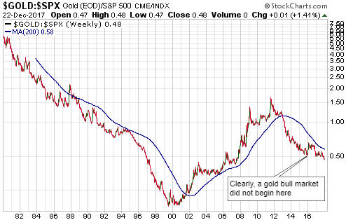
A popular view is that a new cyclical gold bull market commenced in December-2015. If so, the gold bull is now two years old. At the same time, the following weekly chart shows that the gold/SPX ratio (the US$ gold price divided by the S&P500 Index) recently made a 10-year low. Is it possible for gold to be hitting 10-year lows relative to the SPX two years into a gold bull market?

If the sole measuring stick is a depreciating currency then the answer is yes, but if a more practical measuring stick is used then the answer is no.

I explained in an earlier blog post that for a bull-market definition to be practical it must take into account the fact that what people really want from an investment is an increase in purchasing power, not just an increase in price. Unfortunately, it isn’t possible to accurately determine how an investment is doing in purchasing-power terms, but a reasonable alternative is to eliminate the poor measuring stick known as fiat currency from the equation by looking at the performances of different investments relative to each other. The ones that are in bull markets are the ones that are relatively strong.

The definition I arrived at was: An investment is in a bull market if it is in a multi-year upward trend in nominal currency terms AND relative to its main competition.

As also explained in the post linked above, measuring one market against another works especially well for gold bullion and the SPX. This is because they are effectively at opposite ends of an investment seesaw, with the SPX doing best when confidence in money, central banking and government is rising and gold doing best when confidence in money, central banking and government is falling.

I think that it makes no sense to define what happened since December-2015 as a gold bull market. I also think that it is important not to get hung up on bull/bear labels. Bull market or not, January through August of 2016 was a great time to own gold-mining stocks. And bull market or not, the period since August-2016 has been a not-so-great time to be heavily invested in gold-mining stocks.

Rather than being committed to the theory that a gold bull market began in December-2015 or the opposing theory that a gold bear market remains in force, it is better to use sentiment, price action and fundamentals to identify good buying and good selling opportunities in real time.

[This post is an excerpt from a TSI commentary published on 6th December]

The central bank is not the root cause of the boom-bust cycle. The root cause is fractional reserve banking (the ability of banks to create money and credit out of nothing). The central bank’s effect on the cycle is to extend the booms, make the busts more severe and prevent the investment errors of the boom from being fully corrected prior to the start of the next cycle. Consequently, there are some important relationships between interest rates and the performance of the economy that would hold with or without a central bank, provided that the practice of fractional reserve banking was widespread. One of these relationships is the link between a reversal in the yield curve from flattening to steepening and the start of an economic recession/depression.

Unfortunately, the data we have at our disposal doesn’t go back anywhere near as far as we’d like, where “as far as we’d like” in this case means 150 years or more. For example, the data we have for the 10year-2year spread, which is our favourite indicator of the US yield curve, only goes back to the mid-1970s.

For a longer-term look at the performance of the US yield curve the best we can do on short notice is use the Fed’s data for the 10year-3month spread, which goes back to the early-1960s. However, going back to the early-1960s is good enough for government work and is still satisfactory for the private sector.

As explained in many previous commentaries, the boom phase of the cycle is characterised by borrowing short-term to lend/invest long-term in order to take advantage of the artificial abundance of cheap financing enabled by the creation of money and credit out of nothing. This puts upward pressure on short-term interest rates relative to long-term interest rates, meaning that it causes the yield curve to flatten.

At some point, usually after the boom has been in progress for several years, it becomes apparent that some of the investments that were incentivised by the money/credit inflation were ill-conceived. Losses start being realised, the quantity of loan defaults begins to rise, and the opportunities to profit from short-term leverage become scarcer. At this point everything still seems fine to casual observers, central bankers, the average economist and the vast majority of commentators on the financial markets, but the telltale sign that the cycle has begun the transition from boom to bust is a trend reversal in the yield curve. Short-term interest rates begin to fall relative to long-term interest rates, that is, the yield curve begins to steepen.

The following monthly chart of the 10year-3month spread illustrates the process described above. On this chart, the boom periods roughly coincide with the major downward trends (the yield-curve ‘flattenings’) and the bust periods roughly coincide with the major upward trends (the yield-curve ‘steepenings’). The shaded areas are the periods when the US economy was officially in recession.

The black arrows on the chart mark the major trend reversals from flattening to steepening. With two exceptions, such a reversal occurred shortly before the start of every recession.

The first exception occurred in the mid-1960s, when a reversal in the yield spread from a depressed level was not followed by a recession. It seems that something happened at that time to suddenly and temporarily elevate the 10year yield relative to the 3month yield.

The second exception was associated with the first part of the famous double-dip recession of 1980-1982. Thanks to the extreme interest-rate volatility of the period, the yield spread reversed from down to up shortly before the start of the recession in 1980, which is typical, but during the first month of the recession it plunged to a new low before making a sustained reversal.

Due to the downward pressure being maintained on short-term interest rates by the Fed, the yield curve reversal from flattening to steepening that signals an imminent end to the current boom probably will happen with the above-charted yield spread at an unusually high level. We can’t know at what level or exactly when it will happen, but it hasn’t happened yet.