This post has nothing to do with the US Second Amendment or my opinion on whether gun ownership should be legal. It’s about the presentation of gun-related death statistics in a way that supports a political position rather than provides relevant information.
The following chart from a recent post at ritholtz.com compares the number of gun-related deaths to the number of guns per 100 people across many countries. It naturally shows that the country with by far the highest rate of gun ownership (the US) has by far the highest rate of gun-related deaths.
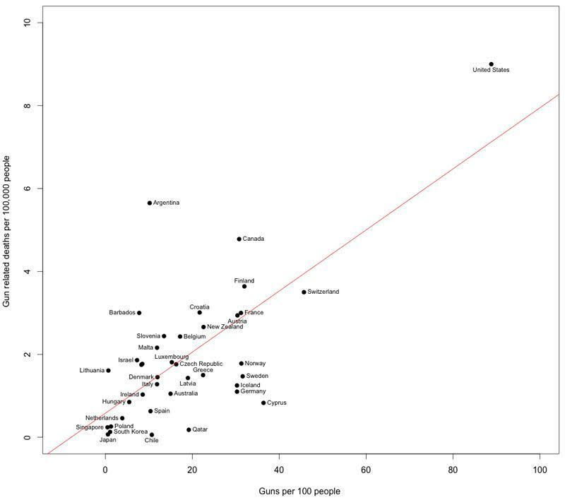
The above chart would be presented for only one reason: to persuade people that the US needs stricter gun control. However, the chart does not make the case for stricter gun control in even a small way. This is because the charted comparison is meaningless.
Obviously, the greater the availability of guns the higher the proportion of gun-related deaths. A country with zero guns will have zero gun-related deaths and a country in which everyone owns a gun will have a significant number of gun-related deaths. This is not evidence that the first country is safer than the second country.
Also, not all gun-related deaths are equal. There is, for example, a huge difference between someone using a gun to take his own life and someone using a gun to take someone else’s life. Lumping all gun-related deaths together is therefore disingenuous. It is part of a deliberate effort to mislead.
The relevant comparison isn’t the gun ownership rate and the gun-related death rate, it’s the gun ownership rate and the total homicide rate or the violent crime rate. Evidence that a higher rate of gun ownership led to a higher rate of homicide and/or a higher rate of violent crime would not prove that stricter gun control was desirable, but at least it would be relevant to the debate.
The following charts from a 2014 article at crimeresearch.org contain relevant information. These charts compare homicide rates and gun ownership rates across countries. They show that the US has a much higher gun ownership rate than average and a slightly higher homicide rate than comparable countries. The slightly higher homicide rate could be due to the higher rate of gun ownership, but it could also be due to other factors.


As mentioned at the start, this post has nothing to do with my opinion on whether the US should have stricter gun control laws. It’s about how statistics are abused to influence opinions and promote agendas.