The following charts relate to an update on the markets that was just emailed to TSI subscribers.

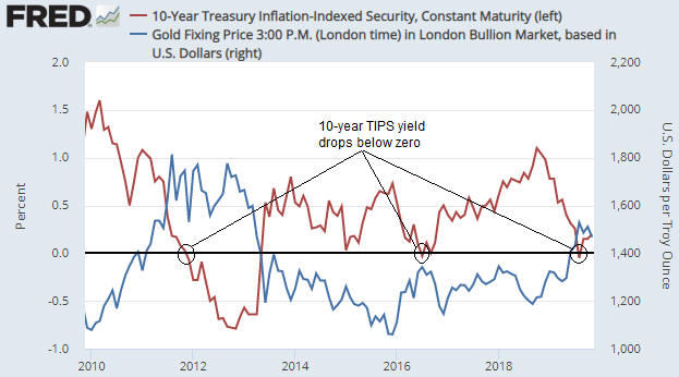
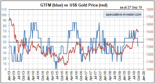
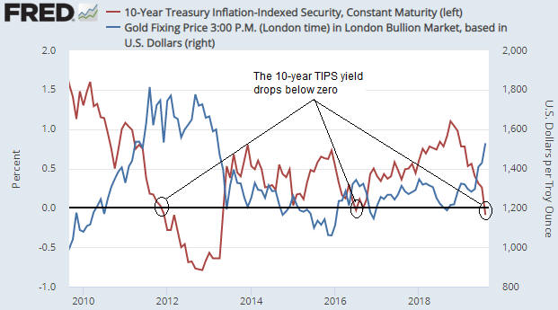
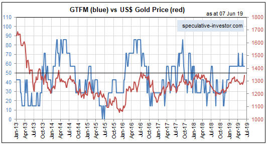
1) Gold

2) The Gold Miners ETF (GDX)

3) The Yen

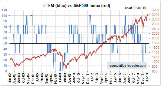
4) The S&P500 Index (SPX)

5) The Russell2000 ETF (IWM)

6) The Dow Transportation Average (TRAN)

7) The iShares 20+ Year Treasury ETF (TLT)

[This blog post is a modified excerpt from a TSI commentary]

In one important respect, the average central banker is like the average politician. They both tend to focus on the direct and/or short-term effects and ignore the indirect and/or long-term effects of policies. In the case of the politician, this is understandable if not excusable. After all, the overriding concern of the average politician is winning the next election. The desire to be popular also influences the decisions of central bankers, but there is a deeper reason for the members of this group’s shortsightedness. The deeper reason is their unwavering commitment to Keynesian economic theory.

All central bankers are Keynesians at heart (if they weren’t they wouldn’t be central bankers), and Keynesian economic theory revolves around the short-term and the superficial. It’s all about policy-makers in the government and the central bank attempting to ‘manage’ the economy by stimulating demand under some conditions and dampening demand under other conditions, with the conditions determined by measures of current or past economic activity. For example, if certain statistics move an arbitrary distance in one direction then an attempt will be made to boost “aggregate demand”. That the concept of “aggregate demand” is bogus is never acknowledged, because acknowledging that the economy comprises millions of distinct individuals as opposed to an amorphous blob would call into question the entire basis for central control of money and interest rates.

In the short-term, the manipulation of money and interest rates often seems to work. In particular, pumping money and forcing interest rates below where they otherwise would be can lead to increased economic activity in the form of more consumption and more investment. What’s happening, however, is that false signals are causing people to make mistakes.

One problem is that people are incentivised by cheaper credit to consume more than they can afford, which guarantees reduced consumption in the future. The bigger problem, though, is on the investment front, in that projects and businesses that would not be financeable at free-market rates of interest are made to appear economically viable. This could seem like a very good thing for a while, but it means that a lot of resources get used in ventures that eventually will fail. It also means that the businesses that would have been viable in a non-manipulated rate environment suffer profit-margin compression due to the ability, created by the abundance of artificially-cheap credit, of relatively inefficient and/or unprofitable competitors to remain in operation.

In addition to the above, the persistent downward manipulation of interest rates leads to huge pension-fund deficits. However, burgeoning shortfalls in the world of pension funds is a major economic and political issue that deserves separate treatment and is outside the scope of this short discussion. Suffice to say right now that the massive unfunded pension liabilities that have arisen due to the policy of interest-rate suppression could be the excuse for new policies that are even more destructive, such as policies based on Modern Monetary Theory (MMT).

Summing up, the policy of interest-rate suppression promotes resource wastage and general profit-margin compression. It therefore reduces economic growth over the long term. Furthermore, it’s not so much that central bankers weigh the long-term cons against the short-term pros and opt for the latter; it’s that their chosen theoretical framework doesn’t even allow them to consider the long-term cons. That’s how the head of the ECB is able to argue with a straight face that even though euro-zone interest rates have been manipulated well into negative territory, more interest-rate suppression is needed to support the economy.

In a blog post in early-September I noted that the 10-year TIPS (Treasury Inflation Protected Security) yield had just gone negative and that the previous two times that this proxy for the real interest rate went negative (August-2011 and July-2016) the gold price was at an important peak. I then attempted to answer the question: If gold tends to benefit from a lower real interest rate, why would the gold price reverse downward shortly after the real interest rate turned negative?

In the earlier post I gave three reasons why a downward reversal in the gold price could coincide with the ‘real’ interest rate going negative. They were:

1) The dip into negative territory marked a low point for the real interest rate.

2) The real interest rate is just one of several fundamental gold-price drivers, so the upward pressure on the gold price exerted by a falling real interest rate could be counteracted by the downward pressure exerted by other fundamental influences.

3) The gold-bullish fundamental backdrop had been fully discounted by the current gold price.

At the time I thought that the third of the above-mentioned reasons may be applicable, because the speculative net-long position in Comex gold futures was very close to an all-time high and the weekly RSI (an intermediate-term momentum indicator) was almost as high as it ever gets.

As it turned out, the first and third reasons were applicable. Sentiment and momentum indicators pointed to extreme enthusiasm for gold on the part of the speculating community, and the following chart, which is an update of the chart included in the blog post linked above, shows that the 10-year TIPS yield reversed upward at the beginning of September.

The current situation is that neither sentiment nor fundamentals are conducive to substantial strength in the gold price. There could be a counter-trend rebound at any time, but the conditions are not right for a resumption of the major upward trend that got underway in the second half of last year.

In an earlier blog post I discussed the relationship between gold and inflation expectations. Contrary to popular opinion, gold tends to perform relatively poorly when inflation expectations are rising and relatively well when inflation expectations are falling.

The relationship outlined above is very clear on the following charts. The first chart shows that over the past 6 years there has been a strong positive correlation between RINF, an ETF designed to move in the same direction as the expected CPI, and the commodity/gold ratio (the S&P Spot Commodity Index divided by the US$ gold price). In other words, it shows that a broad basket of commodities has outperformed gold during periods when inflation expectations were rising and underperformed gold during periods when inflation expectations were falling. The second chart shows the same comparison over the past 12 months. Notice that inflation expectations bottomed for the year (to date) in mid-August and the commodity/gold ratio bottomed about two weeks later.

A large part of the reason for the strong inverse relationship between gold’s relative strength and inflation expectations is the general view that “inflation” of 2%-3% is not just normal, it is beneficial. In fact, most people have been conditioned to believe that it’s a serious economic problem necessitating draconian central bank intervention if money fails to lose purchasing power at a slow and steady pace.

Eventually the rate of “price inflation” will rise to a level where it starts being seen by the public as a major economic problem, and, as a result, the desire to maintain cash savings will enter a steep decline. It is at this point that the relationship depicted above will stop working and the demand for gold will begin to surge in parallel with rising inflation expectations. In other words, at some point the relationship depicted on the above chart will reverse due to declining confidence in the official money. This point probably will arrive within the next 10 years, but probably won’t arrive within the next 12 months. Over the next 12 months it’s likely that gold will continue to be favoured during periods of falling inflation expectations and other commodities will continue to be favoured during periods of rising inflation expectations.

So, if you think that the recent inflation-expectations bounce is the start of a trend then you should be looking for opportunities to increase your exposure to commodities such as oil and copper, not gold. My guess is that inflation expectations bottomed during August-October of this year, but I’m open to the possibility that the bottoming process will extend into early next year.

In a blog post on 30th September I noted that the banking sector (as represented by the US Bank Index – BKX) had begun to show relative strength, a ramification of which was that my Gold True Fundamentals Model (GTFM) had shifted from bullish to bearish. An update is warranted because the situation has changed since then in a way that is both interesting and a little surprising.

Just to recap, the relative performance of the banking sector (as indicated by the BKX/SPX ratio) is an input to my “true fundamentals” models for both the US stock market and the gold market, the difference being that when the input is bullish for one of these markets it is bearish for the other. In particular, relative weakness in the banking sector is considered to be bullish for gold and bearish for general equities.

As explained in the above-linked post, there was enough relative strength in the banking sector during the first half of September to flip the BKX/SPX input from gold-bullish to equity-bullish, causing the GTFM to shift from bullish to bearish. My guess at the time was that the GTFM would return to gold-bullish territory within the next two months, but I pointed out that it is usually better to base decisions on real-time information than on what might happen in the future.

Within a few days of my 30th September post the GTFM shifted back to bullish, where it remains today. This means that apart from a 3-week period during September, the fundamental backdrop has been supportive for gold since the beginning of this year. Refer to the following chart for more detail (the fundamental backdrop is gold-bullish when the blue line on the chart is above 50). Furthermore, there is evidence in the recent price action that gold’s correction is over. However, the fundamental and technical signs of strength in the gold market were not accompanied by signs of weakness in the banking sector.

What’s both interesting and a little surprising is that the renewed signs of strength in gold have gone hand-in-hand with additional signs of strength in the banking sector. Specifically, since my 30th September post the BKX has broken out to the upside (refer to the top section of the following weekly chart) and the BKX/SPX ratio has broken a sequence of declining tops that dates back to early last year (refer to the bottom section of the following chart).

The BKX/SPX ratio is just one of seven inputs to the GTFM, so there are circumstances in which the gold price can trend upward along with relative strength in the banking sector of the stock market. In other words, it isn’t out of the question that over the next few months we will get a gold rally in parallel with a continuing rise in the BKX/SPX ratio and strength in general equities. It’s more likely, however, that the emerging signs of strength in gold are warning of a short-term reversal to the downside in both the broad stock market and the banking sector.

[This post is an excerpt from a recent TSI commentary]

Once an equity bear market is well underway it runs its course, regardless of the Fed’s actions. For example, the Fed started cutting interest rates in January of 2001, but the bear market that began in March of 2000 continued until October-2002. For another example, the Fed started cutting interest rates in September-2007, but a bear market commenced in October-2007 and continued until March-2009 despite numerous Fed actions designed to halt the price decline. On this basis it can be argued that the Fed’s introduction of a new asset monetisation program roughly one week ago won’t prevent the stock market from rolling over into a major bearish trend. However, there is a good reason to think that it could be different this time (dangerous words, we know) and that the Fed’s new money-pumping scheme will prove to be game-changer.

The reason to think that it could be different this time is that in one respect it definitely is different. We are referring to the fact that although the Fed started cutting interest rates in the early parts of the last two cyclical bear markets (2000-2002 and 2007-2009), it didn’t begin to directly add new money to the financial markets until the S&P500 Index had been trending downward with conviction for about 12 months.

To further explain, when the Fed’s targeted interest rates follow market interest rates downward, which is what tends to happen during at least the first half of an economic downturn, the official rate cuts do not add any liquidity to the financial system. It’s only after the Fed begins to pump new money into the financial markets that its actions have the potential to support asset prices.

During the last two bear markets, by the time the Fed started to pump money it was too late to avoid a massive price decline. This time around, however, the Fed has introduced a fairly aggressive money-pumping program while the S&P500 is very close to its all-time high and seemingly still in a bullish trend.

The Fed has emphasised that the new asset monetisation program should not be called “QE” because it does not constitute a shift in monetary policy. Technically this is correct, but in a way it’s worse than a shift towards easier monetary policy. The Fed’s new program is actually a thinly-disguised attempt to help the Primary Dealers absorb an increasing supply of US Treasury debt. To put it another way, the Fed is now monetising assets for the purpose of financing the US federal government, albeit in a surreptitious manner.

This relates to a point we made in a recent blog post. The point is that when the central bank is perceived to be financing the government, as opposed to implementing monetary policy to achieve economic (non-political) objectives such as “price stability”, there is a heightened risk that a large decline in monetary confidence will be set in motion. One effect of this would be an increase in what most people think of as “inflation”.

Summing up, it’s possible that the Fed’s new asset monetisation program will extend the current cycle (prolong the equity bull market) and lead to more “price inflation” than earlier programs.

[This post is a modified excerpt from a recent TSI commentary.]

We regularly look at what’s happening with monetary inflation around the world, but today we’ll focus exclusively on the US monetary inflation rate. This is because of the recent evidence that the unusually-low level of this long-term monetary indicator is starting to have a significant short-term effect.

The following chart shows that the year-over-year rate of change in US True Money Supply (TMS), a.k.a. the US monetary inflation rate, made a new 12-year low in August-2019. Furthermore, the latest TMS growth figure for the US is very close to the 20-year low registered in September-2006.

Within three months of the TMS growth trough in September-2006 the first obvious crack appeared in the US mortgage debt/securitisation bubble. The crack was a trading update issued by HSBC on 5th December 2006 that noted the increasing “challenges” being faced by the Mortgage Services operations of HSBC Finance Corporation. This initial sign of weakness was followed by the appearance of a much larger crack on 7th February 2007. That’s when HSBC issued another trading update that included a profit warning due to substantially increased loan impairment charges. Within days of this February-2007 HSBC update, the shares of sub-prime lending specialists such as New Century Financial and NovaStar Financial went into freefall. This marked the beginning of the Global Financial Crisis, although the US stock market didn’t top out until October of 2007 and industrial commodities such as oil and copper didn’t top out until mid-2008.

The above-mentioned events could be relevant to the current situation, in that the recent chaos in the US short-term funding market could be the initial ‘crack’ in today’s global debt edifice. While the low rate of US monetary inflation was not the proximate catalyst for the recent chaos, there is little doubt that it played a part. Temporary issues such as a corporate tax deadline and a large addition by the US Treasury to its account at the Fed would not have had such a dramatic effect if the money supply had been growing at a ‘normal’ pace.

Generally, when the money supply is growing very slowly within a debt-based monetary system, a relatively small increase in the demand for cash can create the impression that there is a major cash shortage.

Now, if there’s one thing we can be sure of it’s that the next crisis will look nothing like the last crisis. The financial markets work that way because after a crisis occurs ‘everyone’, including all policy-makers, will be on guard against a repeat performance, making a repeat performance extremely improbable. Therefore, we can be confident that even if the recent temporary seizure of the US short-term funding market was a figurative shot across the bow, within the next couple of years there will NOT be a major liquidity event that looks like the 2007-2008 crisis. However, some sort of crisis, encompassing an economic recession, is probable within this 2-year period.

The nature of the next crisis will be determined by how the Fed reacts to signs of economic weakness and short-term funding issues such as the one that arose a few weeks ago. In particular, quick action by the Fed to boost the money supply would greatly reduce the probability of a deflation scare and greatly increase the risk that the next crisis will involve relatively high levels of what most people call “inflation”.

As an aside, there’s a big difference between the Fed cutting its targeted short-term interest rates and the Fed directly boosting the money supply. For example, in reaction to signs of stress in the financial system the Fed commenced a rate-cutting program in September of 2007, but it didn’t begin to directly pump money into the system until September of 2008. In effect, during the last crisis the Fed did nothing to address liquidity issues until almost two years after the appearance of the initial ‘crack’. As a consequence, the monetary inflation rate remained low and monetary conditions remained ‘tight’ until October of 2008 — 12 months after the start of an equity bear market and 10 months after the start of an economic recession.

Early indications are that the Fed will be very quick to inject new money this time around, partly because 2007-2008 is still fresh in the memory. These early indications include the rapidity of the Fed’s response to the effective seizure of the “repo” market last month and the fact that last Friday the Fed introduced a $60B/month asset monetisation program. This program is QE in everything except name. In other words, the Fed already has resumed Quantitative Easing even though GDP is growing at about 2%/year, the unemployment rate is at a generational low and the stock market is near an all-time high.

In summary, while it is too early to have a clear view of how the next major crisis will unfold, something along the lines of 2007-2008 can be ruled out. Also, there are tentative signs that the next crisis will coincide with or follow a period of relatively high “inflation”.

The events of the past 10 years have fostered the belief that central banks can create a virtually unlimited amount of money without significant adverse consequences for the purchasing power of money. Since the law of supply and demand applies to money similarly to how it applies to every other economic good, this belief is wrong. However, the ‘failure’ of QE programs to bring about high levels of what most people think of as inflation has generated a false sense of security.

The difference between money and every other economic good is that money is on one side of almost every economic transaction. Consequently, there is no single number that can accurately represent the price (purchasing power) of money, meaning that even the most honest and rigorous attempt to calculate the “general price level” will fail. This doesn’t imply that changes in the supply of money have no effect on money purchasing power, but it does imply that the effects of changes in the money supply can’t be explained or understood via a simple equation.

Further to the above, the Quantity Theory of Money (QTM) is not a valid theory. Ludwig von Mises thoroughly debunked this theory a hundred years ago and I summarised its basic flaws in a blog post two years ago. Unfortunately, QTM’s obvious inability to explain how the world works has strengthened the belief that an increase in the supply of money has no significant adverse effect on the price of money.

The relationship between an increase in the money supply and its economic effects is complicated by the fact that the effects will differ depending on how and where the new money is added. Of particular relevance, the economic effects of a money-supply increase driven by commercial banks making loans to their customers will be very different from the economic effects of a money-supply increase driven by central banks monetising assets. In the former case the first receivers of the new money will be within the general public, for example, house buyers/sellers and the owners of businesses, whereas in the latter case the first receivers of the new money will be bond speculators (Primary Dealers in the US). Putting it another way, “Main Street” is the first receiver of the new money in the former case and “Wall Street” is the first receiver of the new money in the latter case. This alone goes a long way towards explaining why the QE programs of Q4-2008 onward had a much greater effect on financial asset prices than on the prices that get added together to form the Consumer Price Index (CPI).

Clearly, the QE programs implemented over the past 11 years had huge inflationary effects, just not the effects that many people expected.

A proper analysis of the effects of the QE programs has not been done by central bankers and the most influential economists. As a result, there is now the false sense of security mentioned above. It is now generally believed that substantially increasing the money supply does not lead to problematic “inflation”, which, in turn, lends credibility to monetary quackery such as MMT (Modern Monetary Theory).

Due to the combination of the false belief that large increases in the supply of money have only a minor effect on the purchasing power of money and the equally false belief that the economy would benefit from a bit more “price inflation”, it’s a good bet that central banks and governments will devise ways to inject a lot more money into the economy in reaction to future economic weakness. As is always so, the effects of this money creation will be determined by how and where the new money is added. If the money is added via another QE program then the main effects of the money-pumping again will be seen in the financial markets, at least initially, but if the central bank begins to monetise government debt directly* then the “inflationary” effects in the real economy could be dramatic.

The difference between the direct and the indirect central-bank monetising of government debt is largely psychological, but it is important nonetheless. When the central bank monetises government debt indirectly, that is, via intermediaries such as Primary Dealers, it is perceived to be conducting monetary policy (manipulating interest rates, that is). However, when the central bank monetises government debt directly it is perceived to be financing the government, thus eliminating any semblance of central bank independence and potentially setting in motion a large decline in monetary confidence.

According to the book Monetary Regimes and Inflation, ALL of the great inflations of the 20th Century were preceded by central bank financing of large government deficits. Furthermore, in every case when the government deficit exceeded 40% of expenditure and the central bank was monetising the bulk of the deficit, a period of high inflation was the result. In some cases hyperinflation was the result.

In summary, growth in the money supply matters, but not in the simplistic way suggested by the Quantity Theory of Money. There’s a good chance that this fact will be rediscovered within the next few years, especially if legislative changes enable/force the Fed to monetise government debt directly.

*In the US this would entail the Fed paying for government debt securities by depositing newly-created dollars into the government’s account at the Fed. The government would then spend the new money. Currently the Fed buys government debt securities from Primary Dealers (PDs), which means that the newly-created dollars are deposited into the bank accounts of the PDs.

One of the past month’s interesting stock-market developments was the strength of the banking sector in both nominal terms and relative to the broad market. The strength in nominal dollar terms is illustrated by the top section of the following weekly chart, which shows that the US Bank Index (BKX) is threatening to break out to the upside. The strength relative to the broad market is illustrated by the bottom section of the chart, which reveals a sharp rebound in the BKX/SPX ratio since the beginning of September.

Bank stocks tend to perform relatively well when long-term interest rates are rising in both absolute terms and relative to short-term interest rates. This explains why the banking sector outperformed during September and also why bank stocks generally have been major laggards since early last year.

Valuations in the banking sector are depressed at the moment, as evidenced by relatively low P/Es and the fact that the BKX/SPX ratio is not far from a 25-year low. This opens up the possibility that we will get a few quarters of persistent outperformance by bank stocks after long-term interest rates make a sustained turn to the upside.

On a related matter, the relative performance of the banking sector (as indicated by the BKX/SPX ratio) is an input to my “true fundamentals” models for both the US stock market and the gold market. However, when the input is bullish for one of these markets it is bearish for the other. In particular, relative weakness in the banking sector is considered to be bullish for gold and bearish for general equities.

Until recently the BKX/SPX input was bullish in my gold model and bearish in my equity model, but there was enough relative strength in the banking sector during the first half of September to flip the BKX/SPX input from gold-bullish to equity-bullish. As a consequence, during the second week of September there was a shift from bullish to bearish in my Gold True Fundamentals Model (GTFM). This shift is illustrated on the following weekly chart by the blue line’s recent dip below 50.

The upshot is that the fundamental backdrop, which was supportive for gold from the beginning of this year through to early-September, is now slightly gold-bearish. My guess is that it will return to gold-bullish territory within the next two months, but in situations like this it is better to base decisions on real-time information than on what might happen in the future.

[This blog post is an excerpt from a commentary published at TSI on 1st September 2019.]

It’s well known that the US$ gold price often trends in the opposite direction to the US real interest rate. This relationship is illustrated by the following chart in which the real interest rate is represented by the yield on the 10-year TIPS (Treasury Inflation Protected Security).

Notice that the 10-year TIPS yield has just gone negative and that the previous two times that this proxy for the real interest rate went negative the gold price was at an important peak. Specifically, the real interest rate going negative in August-2011 coincided with a long-term top in the gold price and the real interest rate going negative in July-2016 coincided with an intermediate-term top in the gold price. If gold tends to benefit from a lower real interest rate, why would the gold price reverse downward shortly after the real interest rate turned negative?

Considering only the 2016 case the answer to the above question seems obvious, because in July-2016 the TIPS yield reversed course and began trending upward soon after it dipped into negative territory. In other words, the downward reversal in the gold price coincided with an upward reversal in the real interest rate. However, in 2011-2012 the real interest rate continued to trend downward for more than a year after the gold price peaked.

We think there are two reasons why the gold price didn’t make additional gains in 2011-2012 after the real interest rate turned negative. First and foremost, the real interest rate is just one of several fundamental gold-price drivers (the 10-year TIPS yield is one of seven inputs to our Gold True Fundamentals Model), and after August-2011 the upward pressure exerted by a falling real interest rate was counteracted by the downward pressure exerted by other fundamental influences. Second, in August-2011 a further significant decline in the real interest rate had been factored into the current gold price.

The risk at the moment is that on a short-term basis the bullish fundamental backdrop, including the potential for a further decline in the ‘real interest rate’, is fully discounted by the current price. This risk is highlighted by the fact that the total speculative net-long position in Comex gold futures is very close to an all-time high. It is also highlighted by the fact that the RSI displayed in the bottom section of the following weekly chart is almost as high as it ever gets.

The relationship between short-term market interest rates and the interest rates set by the Fed is a complicated one. The market makes predictions about what the Fed is going to do and moves in anticipation, but at the same time the Fed’s interest-rate settings are influenced by what’s happening to market interest rates. Also, market interest rates are determined by factors other than what the Fed is doing or expected to do to its official rate targets, and as a result there are times when the market and the Fed seem to be at odds with each other.

At the moment there is no doubt that the market is leading the Fed. In particular, the Fed has been swayed towards rate cutting partly by the fact that the market has discounted rate cuts. This can be established by comparing recent movements in market interest rates with changes in the Fed’s interest rate targets, which I’ll get to shortly. It can also be established by referring to the Fed’s own statements. For example, the minutes of the July FOMC meeting included the following assessment:

“Participants observed that current financial conditions appeared to be premised importantly on expectations that the Federal Reserve would ease policy to help offset the drag on economic growth stemming from the weaker global outlook and uncertainties associated with international trade as well as to provide some insurance to address various downside risks.”

In essence, the Fed has admitted here to being worried that if it doesn’t cut rates like the market expects then financial conditions could get a lot worse. The implication is that if the market expects the Fed to cut rates, then to avoid disappointing the market (and risking the deterioration of financial conditions) the Fed will cut rates.

I mentioned above that the market’s current leadership can be established by comparing recent movements in market interest rates with changes in the Fed’s interest rate targets. Displayed below is a chart that makes this case. The chart shows the performance of the 2-year Treasury yield and indicates the last two interest-rate changes made by the Fed. Notice that:

1) The 2-year market interest rate began trending downward in early-November of 2018.

2) The Fed made its last rate hike during the second half of December 2018, that is, the Fed was still in rate-hiking mode six weeks after a short-term market interest rate began trending downward.

3) The Fed made its first rate cut at the end of July 2019. By that time, the 2-year market interest rate had been trending downward for almost 9 months.

It’s reasonable to assume that additional Fed rate cuts are on the way. Bear in mind, however, that a few additional rate cuts have already been factored into market prices, so market prices won’t necessarily respond in the obvious way to future Fed rate cuts. Also bear in mind that market interest rates probably will begin trending upward while the Fed and other central banks are still in rate-cutting mode.

[This post is a modified excerpt from a recent TSI commentary]

Gold tends to lead the industrial metals sector at intermediate-term bottoms, that is, the US$ gold price tends to make an intermediate-term bottom and commence a multi-quarter (or multi-year) upward trend in advance of the Industrial Metals Index (GYX). Evidence of this can be found on the following chart comparison of the US$ gold price and GYX. Specific examples are:

a) The gold price reversed upward in April of 2001 and GYX did the same in November of that year.

b) The gold price reversed upward in October-November of 2008 and GYX did the same in February-March of 2009.

c) The gold price reversed upward in December of 2015 and GYX followed suit in January of 2016.

Gold’s most recent intermediate-term bottom was in August of 2018. It has since trended upward and over the past two months the trend accelerated. GYX, however, continued to make lower lows until June of 2019. It’s too early to tell if GYX’s June-2019 low was the intermediate-term variety, but regardless of whether or not it makes a new low within the next couple of months the performance of the gold market suggests that the industrial metals sector will commence an intermediate-term rally before the end of this year.

The Baltic Dry Index (BDI) is also predicting an industrial metals rally

The BDI is an index of dry bulk shipping rates. I generally don’t use it as an economic or a financial-market indicator, because it is influenced as much by changes in the supply of shipping capacity as by changes in the global demand for commodities. However, intermediate-term trends in the BDI often match intermediate-term trends in the Industrial Metals Index (GYX). Also, large short-term divergences between the BDI and GYX tend to be important, with one or the other subsequently making a big catch-up move in quick time.

As illustrated by the following chart, a large divergence has opened up over the past four months due to the BDI rocketing up to a 5-year high while GYX languishes near a 2-year low. This divergence could be closed by either a dramatic plunge in the BDI or a substantial rally in the industrial metals sector. I suspect it will be the latter.

The euro may well gain in value relative to the US$ over the next 12 months, but three differences between the monetary systems of the US and the euro-zone guarantee that the euro will collapse (cease being a useful medium of exchange) before the US$ collapses.

The first difference is to do with the euro-zone system being an attempt to impose common monetary policy across economically and politically disparate countries. This is a problem. A central planning agency imposing monetary policy within a single country is bad enough because it generates false price signals and in so doing reduces the rate of economic progress. However, when monetary policy (the combination of interest-rate and money-supply manipulations) is implemented across several economically-diverse countries the resulting imbalances grow and become troublesome more quickly.

As an aside, money is supposed to be a medium of exchange and a yardstick, not a tool for economic manipulation. Therefore, it is inherently no more problematic for different countries to use a common currency than it is for different countries to use common measures of length or weight. On the contrary, a common currency makes international trading and investing more efficient. For example, there were long periods in the past when gold was used simultaneously and successfully as money by many different countries. However, if a currency can be created out of nothing then there is no getting around the requirement to have an institution that oversees/manages it. The euro therefore could not be ‘fixed’ by simply eliminating the ECB. The ECB and the one-size-fits-all monetary policy it imposes are indispensable parts of the euro-zone system.

The second difference is linked to the concept that a government with a captive central bank cannot become insolvent with respect to obligations in its own currency. For example, due to the existence of the Fed the US government will always have access to as much money as it needs to meet its obligations, regardless of how much debt it racks up. Putting it another way, should all other demand for Treasury debt disappear the Fed will still be there to monetise whatever amount of debt the US government issues. Consequently, the US government will never be forced to directly default on its debt.

It’s a different story in the euro-zone, however, because the ECB is not beholden to any one government. The provision of ECB financial support to one euro-zone government therefore requires the acquiescence of other governments. This hasn’t been a stumbling block to date and the ECB has provided whatever support was needed to prevent financially-stressed euro-zone governments from directly defaulting on their debts, but eventually a point will be reached when the governments of some countries balk at their interest rates and money being distorted as part of an effort to prop-up the finances of other governments. At that point there will be direct default on euro-zone government debt or the disintegration of the monetary union.

Once it becomes clear that direct default on government debt is a risk to be reckoned with, ‘capital’ will flee the euro-zone at a rapid rate. This is because the main (only?) reason to own government bonds is that they are supposedly risk free.

The third critical difference between the US and euro-zone monetary systems is similar to the second difference. In the US there is a symbiotic relationship between the Fed and the government, with one institution always prepared to support the other in a time of crisis. One consequence of this relationship is the impossibility — as discussed above — of the US government ever being forced to directly default on its debt. Another consequence is the impossibility of the Fed ever becoming bankrupt.

Several years ago there was much speculation that the Fed would go broke due to large losses on the bonds it was buying in its QE operations, but this speculation was never well-informed. Up until now the Fed has made out like the bandit it is on its ‘investments’ in Treasury and mortgage-backed securities, but even if these securities had collapsed in value it would not have resulted in the Fed going bust. It simply would have led to a line being added to the Fed’s balance sheet to keep the books in balance.

Again, though, it’s a different story in the euro-zone. Should the ECB begin to incur large losses on its bond portfolio there is no certainty that it would be able to keep going about its business as usual. To do so would require the support of governments/countries that never benefited from and never whole-heartedly agreed with the programs that led to the pile-up of low-quality bonds on the ECB’s balance sheet.

Summing up, the US monetary system is problematic in that it gets in the way of economic progress, but it is much less fragile than the euro-zone monetary system. That’s why the euro-zone system will be the first to collapse.

Below is an excerpt from a recent TSI commentary.

An investment’s true fundamentals exert pressure on its price. It is not unusual for the price to trend in the opposite direction to the fundamentals for a while, but if fundamentals-related pressure consistently acts in one direction then the price should eventually fall into line by trending in that direction. Our “true fundamentals” models for gold, the US stock market, the Dollar Index and commodities (the GSCI Commodity Index) are attempts to quantify the magnitude and direction of fundamentals-related pressure.

We have a lot of confidence in our Gold True Fundamentals Model (GTFM), because we understand why it should work and we know that it has worked well over a long enough period to rule out luck/randomness. It isn’t a short-term timing indicator, but all intermediate-term trends in the US$ gold price over the past 17 years* have been in line with the fundamentals as reflected by the GTFM. However, we have less confidence in our other true fundamentals models.

We recently have given more thought to the construction of our Equity True Fundamentals Model (ETFM), which is designed to indicate the direction and magnitude of fundamentals-related pressure on the US stock market (as represented by the S&P500 Index).

The version of the ETFM that we have been using takes into account credit spreads, the yield curve, the real interest rate (as indicated by the 10-year TIPS yield), the relative strength of the banking sector and the G2 monetary inflation rate, with the monetary inflation rate given a greater weighting than the other inputs. However, we now think it was a mistake to put extra emphasis on monetary inflation. This is because although the rate of change in the money supply is the most important long-term driver of the stock market, the time between a trend change in monetary inflation and the effects of this trend change becoming evident in the stock market is long and variable.

In an effort to make the ETFM more useful over the intermediate-term (6-18 month) periods that are of primary interest to us we have made two changes to the Model’s construction. First, we have reduced the emphasis on monetary inflation so that it has the same weighting as the Model’s other inputs. Second, the ISM New Orders Index (NOI) has been added as an input to the Model. This input will be set to 1 when the NOI is 55 or above and set to 0 when the NOI is below 55. This is being done because a) the stock market tends to perform much better when the NOI is greater than 55 than when the NOI is less than 55, and b) there is a strong tendency for the NOI to fall below 55 PRIOR to periods of significant stock market weakness, meaning that weakness in the NOI is not simply a reaction to weakness in the stock market.

The above changes didn’t make a big difference to the historical performance of the ETFM, but they did make the Model a little more sensitive to shifts in the fundamental winds. This is a plus, because the original model wasn’t sensitive enough. Note, as well, that these changes did not alter the current signal. Both the original ETFM and the new/improved ETFM switched from neutral to bearish on 19th April 2019.

Here is a chart comparing the new ETFM (the blue line) with the SPX since the start of 2002. Stock market fundamentals are considered to be bearish when the ETFM is below 50, neutral when the ETFM equals 50 and bullish when the ETFM is above 50.

The true fundamentals are equity-bearish at the moment. If they remain bearish then the price eventually WILL fall into line. Furthermore, the longer the price trends upward or stays elevated in parallel with a bearish fundamental backdrop, the faster the eventual downward price move is likely to be.

*For some of the GTFM inputs we don’t have data prior to the early-2000s, so we can’t compare the GTFM and the gold price during earlier periods.

There is no simple relationship between interest rates and the stock market. In particular, a lower interest rate doesn’t necessarily lead to a higher stock market and a higher interest rate doesn’t necessarily lead to a lower stock market.

The conventional wisdom on this topic is based largely on what happened over the past few decades. Clearly, US equities generally fared well after interest rates embarked on a long-term downward trend in the early 1980s and generally fared poorly when interest rates were in a rising trend during the 10-14 year period prior to the early 1980s. Also, the inverse relationship (a lower interest rate leads to a higher stock market and a higher interest rate leads to a lower stock market) seemed to make sense and was incorporated into a popular stock market valuation tool called “The Fed Model”.

The Fed Model compares the earnings yield of the S&P500 Index (the reciprocal of the S&P500′s P/E ratio, expressed as a percentage) with the 10-year T-Note yield to determine if the stock market is over-valued or under-valued. The higher the S&P500 yield relative to the 10-year T-Note yield, the better the value supposedly offered by the stock market. An implication is that if the 10-year yield is very low, the S&P500 can have a very high P/E ratio and still not be over-valued. For example, according to the Fed Model the S&P500 is attractively valued today. This is because even though the current P/E ratio is almost as high as it ever gets (excluding the 1999-2000 bubble period), the current earnings yield is well above the current 10-year T-Note yield.

However, the simple relationship between interest rates and the stock market only makes sense at a superficial level. It doesn’t hold up under deeper analysis. The reason is that the current value of a company is the sum of all of that company’s future cash flows discounted at some rate, and in most cases it will not be appropriate to use today’s interest rate to discount cash flows that won’t happen until many years or even decades into the future.

When picking a rate at which to discount distant cash flows it would be more reasonable to use a long-term average interest rate than to use the current interest rate. Furthermore, there is no good reason why the change in the interest rate over the next 12 months should significantly affect the interest rate used to discount cash flows that are expected to occur 10-20 years into the future.

But if it is wrong to assume that the stock market should trend inversely to the interest rate over long periods, then why did this assumption prove to be correct over the bulk of the past 50 years?

The first part of the answer is that over the very long term the stock market swings from under-valued to over-valued and back again and that in the early 1980s a bond market under-valuation extreme happened to coincide with a stock market under-valuation extreme. The second part of the answer is that financial market history goes back much further than 50 years and the simple relationship on which the Fed Model is based is not apparent prior to 1970. In essence, the theory that a lower interest rate leads to a higher stock market and a higher interest rate leads to a lower stock market is an artifact of the past 50 years.

The above statement is supported by the following charts. The charts show the Dow Industrials Index and the 10-year T-Note yield from the beginning of 1925 through to the end of 1968.

The US stock market (as represented by the Dow Industrials in this case) was in a secular bearish trend from 1929 until 1942. Apart from an upward spike due to fear of government default in 1931, the 10-year yield was in a downward trend during this bearish stock market period. The stock market then embarked on a secular bullish trend that didn’t end until the late-1960s. The 10-year yield was in an upward trend during this bullish stock market period. That is, the long-term relationship between interest rates and the stock market during 1929-1968 was the opposite of what it was over the past 50 years.

A large divergence between two fundamentally-correlated market prices is important because such a divergence usually will be closed via a big move in one or both prices. However, divergences sometimes build for an inconveniently long time before they start to matter.

The gold/commodity ratio (the US$ gold price divided by the GSCI Spot Commodity Index) and the T-Bond are strongly correlated over the long term. They also tend to be well correlated over shorter timeframes, but significant short-term divergences sometimes occur. One such divergence has been developing since the beginning of this year, with the T-Bond making a sequence of higher highs while the gold/commodity ratio stays below its late-December high. Note that even the recent surge to a new 5-year high by the US$ gold price was not enough to push the gold/GNX ratio above its late-December high.

The current divergence and previous similar divergences (higher highs for the T-Bond in parallel with lower highs for the gold/commodity ratio) are illustrated by the following chart. The previous similar divergences led to large declines in the T-Bond price and I can think of no reason to expect that it will be different this time.

[This post is an excerpt from a recent TSI commentary]

Gold tends to perform well relative to commodities in general when inflation expectations are FALLING. The evidence is presented below in chart form.

The first of the following charts shows the Expected CPI, which in this case is determined by subtracting the yield on the 5-year TIPS (Treasury Inflation Protected Security) from the yield on the 5-year T-Note. In effect, the chart shows the average annual “inflation” rate that the market expects the US government to report over the next 5 years. We’ve labeled all of the important highs and lows on this chart.

The second of the following charts shows the gold/commodity ratio (the US$ gold price divided by the GSCI Spot Commodity Index). The labels on this chart correspond to the labels on the first chart. For example, point A on the first chart is the same time as point A on the second chart.

Notice that in every case over the 6-year period covered by the following charts, a high for inflation expectations (the Expected CPI) is associated with a low for the gold/commodity ratio and a low for inflation expectations is associated with a high for the gold/commodity ratio.

The relationship we tried to show above is more clearly demonstrated by the next chart. On this chart the commodity/gold ratio (as opposed to the gold/commodity ratio) is compared to the ProShares Inflation Expectations ETF (RINF). The correlation clearly is strong, with commodities consistently outperforming gold when inflation expectations are rising and underperforming gold when inflation expectations are falling.

An implication of the above charts is that if inflation expectations are close to an intermediate-term bottom then the financial world is close to the start of a 6-12 month period during which the industrial metals perform better than gold. Alternatively, a further decline in inflation expectations (increasing fear of deflation) would lead to additional relative strength in gold.

We realise that the above message is the opposite of what most people believe about gold, but a lot of what most people believe about gold is not accurate. Of particular relevance to this discussion, gold has never been a hedge against “price inflation”.

Gold tends to perform relatively well during periods when financial-system and/or economic confidence is on the decline. The declining confidence sometimes will go hand-in-hand with rapid “price inflation”, but it isn’t reasonable to expect gold to be a useful hedge against what generally is considered these days to be normal “inflation”. In fact, part of the reason for the strong INVERSE relationship between the gold/commodity ratio and inflation expectations is the general view that “inflation” of 2%-3% is beneficial.

Our view is that the next three months could be dicey, especially if there’s another sharp decline in the stock market. However, we think that by the end of this year inflation expectations will be significantly higher and industrial metals such as copper and platinum will be significantly more expensive relative to gold.

[This post is a slightly-modified excerpt from a TSI commentary published about two weeks ago.]

The way that most new money was created over the past 10 years was different to how it was created during earlier cycles. During earlier cycles almost all new money was loaned into existence by commercial banks, but in the final few months of 2008 the Fed stopped relying on the commercial banks and began its own money-creation program (QE).

The difference is important because most of the money created by commercial banks is injected into the ‘real economy’ (the first receivers of the new money are businesses and the general public), whereas all of the money created by the Fed is injected into the financial markets (the first receivers of the new money are bond traders). The Fed’s new money eventually will find its way to Main Street (as opposed to Wall Street), but the rate of monetary inflation experienced by the ‘real economy’ during the years following the Global Financial Crisis was a lot lower than suggested by the change in the US True Money Supply (TMS). Consequently, there may have been a lot less mal-investment during the current cycle than during the years leading up to the 2007-2009 crisis.

Don’t get us wrong — there has been a huge amount of ill-conceived and misdirected investment due to the Fed’s money-pumping and associated suppression of interest rates. Due to these bad investments, corporate balance sheets are now much weaker, on average, than otherwise would be the case. In particular, the corporate world collectively has gone heavily into debt and in a lot of cases the debt has not been used productively. For example, it has been used to buy back shares or fund high-priced acquisitions. This will have very negative consequences for the stock market within the next few years, but wasting money on share buy-backs and over-paying for assets does not cause the business cycle.

The ‘boom’ phase of the business cycle happens when artificially-low interest rates prompt investment, on an economy-wide scale, in new production facilities and construction projects that would not have seemed viable in the absence of the distorted interest-rate signal. The ‘bust’ phase of the business cycle kicks off when it starts to become apparent that, due to rising construction/production costs and/or less consumer demand than forecast, the aforementioned investments either cannot be completed or will generate a lot less cash than originally expected. Widespread liquidation ensues, and — as long as policy-makers don’t do too much to ‘help’ — resources eventually get reallocated in a way that meshes with sustainable consumer demand. The economy recovers.

The above is background information for the following charts. The first chart shows the year-over-year (YOY) rate of change in US True Money Supply (TMS), a.k.a. the US monetary inflation rate. The second chart shows the US monetary inflation rate without the Fed’s direct additions and deletions*.

Note that the second chart does not show what would have happened to the US monetary inflation rate in the absence of the Fed. Regardless of whether the Fed is creating new money or not, it exerts a strong influence on the commercial banks. What we have tried to do with the second chart is isolate the monetary inflation that causes the business cycle.

Prior to late-2008 the charts are very similar, but from late-2008 onwards there are some big divergences. The most obvious divergence was in 2009, when the rate of growth in TMS extended the rapid upward trend that began in 2008 while the rate of growth in “TMS minus Fed” collapsed to well below zero. Also worth mentioning is that the rate of growth in “TMS minus Fed” was in negative territory from August-2013 to June-2014, a period during which the rate of growth in TMS never dropped below 7%.

The swings in the “TMS minus Fed” growth rate explain some of the important swings in the US economy. For example, the rapid increase in “TMS minus Fed” during 2011-2012 almost certainly is linked to the mad rush to invest in the shale oil industry, and the 2013-2014 plunge in “TMS minus Fed” would be partly responsible for the collapse of the shale-oil investment boom during 2014-2015. Although it was focused on a single industry, this was a classic case of the mal-investment that results in a boom-bust cycle.

Over the past 18 months the TMS growth rate has extended its major downward trend, but the “TMS minus Fed” growth rate has rebounded. This rebound could delay the start of a recession.

*We assume that the amount of money added by the Fed equals the increase in the Fed’s holdings of securities minus the increase in Reverse Purchase Agreements.

After spending almost all of 2018 in bearish territory, gold’s true fundamentals* (as indicated by my Gold True Fundamentals Model – GTFM) have spent all of this year to date in bullish territory. Refer to the following chart comparison of the GTFM (the blue line) and the US$ gold price (the red line) for the details.

A market’s true fundamentals are akin to pressure. Due to sentiment and other influences a market can move counter to the fundamentals for a while, but if the fundamentals continue to act in a certain direction then the pressure will build up until the price eventually falls into line. Also, even if it isn’t sufficient to bring about a significant rally, the upward pressure stemming from a bullish fundamental backdrop will tend to create a price floor. That’s what happened with gold during March and April.

As was the case when I last addressed this topic at the TSI Blog, the most important GTFM input that is yet to turn bullish is the yield curve (as indicated by the 10year-2year and 10year-3month yield spreads). This input shifting from bearish to bullish requires a reversal in the yield curve from flattening (long-term rates falling relative to short-term rates) to steepening (long-term rates rising relative to short-term rates). If the reversal is driven primarily by falling short-term interest rates it indicates a boom-to-bust transition, such as occurred in 2000 and 2007, whereas if the reversal is driven primarily by rising long-term interest rates it points to increasing inflation expectations.

As illustrated below, at the end of last week there was no evidence of such a trend change in the 10year-3month yield spread.

To get a gold bull market there probably will have to be a sustained trend reversal in the yield curve. I think that will happen during the second half of this year, but it hasn’t happened yet. Also, when it does happen my guess is that it will be driven by rising long-term interest rates (indicating rising inflation expectations), not falling short-term interest rates. That’s an out-of-consensus view right now, because inflation expectations are low/falling and almost everyone has come to the conclusion that an aggressive Fed rate-cutting campaign will get underway in the near future.

Another GTFM input that could shift from bearish to bullish in the near future and thus add to the upward pressure on the gold price is the currency exchange rate input. At the moment, all it would take to bring about this shift is a weekly close in the Dollar Index about half a point below last week’s close.

My guess is that there will be some corrective activity in the gold market over the coming 1-2 weeks, but as long as the GTFM stays in bullish territory the fundamentals-related upward pressure should enable the gold price to make new multi-year highs within the next few months.

*I use the term “true fundamentals” to distinguish the actual fundamental drivers of the gold price from the drivers that are regularly cited by gold-market analysts and commentators. According to many pontificators on the gold market, gold’s fundamentals include the volume of metal flowing into the inventories of gold ETFs, China’s gold imports, the volume of gold being transferred out of the Shanghai Futures Exchange inventory, the amount of “registered” gold at the COMEX, India’s monsoon and wedding seasons, jewellery demand, the amount of gold being bought/sold by various central banks, changes in mine production and scrap supply, and wild guesses regarding JP Morgan’s exposure to gold. These aren’t true fundamental price drivers. At best, they are distractions.

In 1961, Deng Xiao Ping uttered what is perhaps his most famous quotation: “I don’t care if it’s a white cat or a black cat. It’s a good cat so long as it catches mice.” This was interpreted to mean that being economically successful is more important than being loyal to any particular ideology.

Deng’s view that having a productive economy was more important than adhering rigidly to theories that were failing in practice brought him into conflict with Mao Tse Tung. It could be argued that Deng was more practical than Mao in that he was prepared to allow/encourage some elements of a market economy, although if the primary objective is holding onto political power then what’s practical is not necessarily what’s best for the country.

From a purely political perspective, Mao was practical. His policies generally had disastrous economic effects, but in addition to maintaining power he was able to stay popular with China’s peasant class (his political support base). He did this by creating the impression that there was always a revolution — of one form or another — to be fought. There were always enemies that had to be defeated, mountains that had to be climbed and sacrifices that had to be made in the present in order to set the stage for a brighter future.

The revolutionary feeling was sustained via a series of dramatic programs and policy shifts, chief among them being:

1. “The Hundred Flowers Campaign” of 1956-1957: Mao encouraged differing opinions on how China should be governed and even permitted public criticism of the Communist Party leadership.

2. “The Anti-Rightist Movement” of 1957-1959: Those who accepted Mao’s invitation to express anti-communist opinions under the “Hundred Flowers Campaign” were eliminated (purged, imprisoned, killed). Quite likely, the “Hundred Flowers Campaign” was just a ruse to identify anyone who could possibly be a threat to Mao.

3. “The Great Leap Forward” of 1958-1962: A 5-year plan focusing on the collectivisation of agriculture that caused widespread food shortages and resulted in the death of tens of millions of people (estimates of the famine-related death toll range from 20M to 45M). This disaster created the first serious rift between Mao and Deng, which eventually led to Deng being purged from the Communist party in the early days of the “Cultural Revolution”.

4. “The Cultural Revolution” of 1966 through to Mao’s death in 1976: Ostensibly a movement to topple the “ruling class”, spread power more evenly and stamp out counter-revolutionary activities, this was Mao’s most blatant attempt to keep China in a perpetual state of revolution. During the “Cultural Revolution”, anyone considered to have skills above those of the average person became a likely target for persecution. In addition, formal education all but ceased, countless works of art and historical buildings were destroyed, and Mao’s “Little Red Book” of quotations effectively became the bible. The result was social and economic chaos.

Fortunately for China, Deng was able to gain control of the Communist Party following Mao’s death. The reforms he implemented showed that even a modicum of economic freedom can go a long way towards improving living standards.

Interestingly, one of the most successful reforms of the Deng era was not the brainchild of Deng, but was, instead, developed by local farmers who were desperate to escape the poverty that collectivised agriculture had imposed upon them. In much the same way that America’s Pilgrims adopted private ownership of farmland in response to a communal system’s failure to produce sufficient food, the inhabitants of one small Chinese village decided, in 1978, to experiment with a new system under which individuals and families would have ownership of farmland. The experiment was a huge success, and was subsequently tried — also with great success — in some other villages. After learning of these experiments and the resultant large increases in agricultural productivity, Deng openly praised the participants and encouraged the nationwide adoption of the ‘new’ system. It is almost certain that the government’s reaction would have been very different if Mao had still been in power.

China’s political leaders between Deng Xiao Ping and Xi Jin Ping, the current leader, were really just place fillers. It’s clear that Xi is the most important leader of the Communist Party of China (CPC) since Deng.

Xi seems to be more like Mao than Deng, in that he places the supremacy of the Party above all other considerations and puts a strong emphasis on Communist ideology. He has made this clear in numerous speeches. For example:

At the October 2017 19th Party Congress, he said: “Government, military, society and schools, north, south, east and west, the Party is the leader of everything.”

And in March-2018, Xinhua (China’s official state-run press agency) quoted him as saying: “The Party exercises overall leadership over all areas of endeavor in every part of the country. A primary task of deepening reform of the Party and state institutions is to strengthen the CPC’s leadership in every sector.”

The phrase “capitalism with Chinese characteristics” is not used in China, at least not by any high-ranking members of the CPC. Only Western pundits believe that China is shifting towards capitalism. In China the political system is often referred to as “socialism with Chinese characteristics”. Here are two examples from a Xi speech given last year at the Central Commission for Discipline Inspection (CCDI) Plenary Session:

“[Party members should] understand the dialectical relationship between the grand vision of Communism and socialism with Chinese characteristics.”

“We cannot indulge ourselves in empty talk without working for the cause of socialism with Chinese characteristics and national rejuvenation. We can neither afford to lose the grand vision because realizing Communism is a long process.”

And here’s an excerpt from a Xinhua article that quotes Xi making the same point:

“The purpose of reviewing the Communist Manifesto is to understand and grasp the power of the truth of Marxism and write a new chapter of socialism with Chinese characteristics in the new era, Xi said. It’s necessary to “apply the scientific principles and the spirit of The Communist Manifesto to the overall planning of activities related to the great struggle, great project, great cause, and great dream,” he said. More efforts should be made to develop Marxism in the 21st century and in contemporary China, and write a new chapter of adapting Marxism to the Chinese context, Xi said.”

Like Mao, Xi is attempting to galvanise support behind himself and the Party (Xi is now defined as the “core” of the Party) by promoting the idea that China and the Chinese people are under threat. In this regard he is being helped by having a ready-made enemy in the form of a US government that clearly is trying to contain China both economically and militarily. Moreover, the “trade war” and the US government restrictions on US corporations doing business with Huawei make Xi look prescient, because he has warned for many years that this sort of thing could happen and therefore that it was dangerous for Chinese manufacturers to rely on imported technology.

Unfortunately for Xi, innovation, which he correctly perceives to be lacking in China, won’t happen at the command of government.

Also like Mao, Xi does not tolerate any dissension. All views must be consistent with the goal of having a population unified in its beliefs in “socialism with Chinese characteristics” and the primacy of the Party in all aspects of life. Hence the draconian treatment of millions of Muslims in Xinjiang Province, the severe policing of opinions expressed in social media and the setting-up of the world’s largest domestic surveillance network.

In a way, China has come full circle. However, Xi has far greater technological and economic resources at his disposal than Mao could have ever dreamed of.